
拳皇十周年纪念版无限气下载
alicucu 2026-01-19 10:32 33 浏览
下载一个啪啪模拟器在里面找有很多拳皇包括十周年而且里面有干枯大地七枷社
浏览器搜索游戏名、打开相关网站的网页、可以下载游戏安装文件!!
1.
以win10,谷歌浏览器为例。
打开谷歌浏览器

2.
浏览器地址栏输入网址https://down.ali213.net/pcgame/kof14.html

3.
点击资源检索

4.
点击电信高速下载
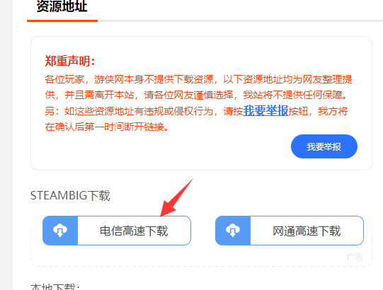
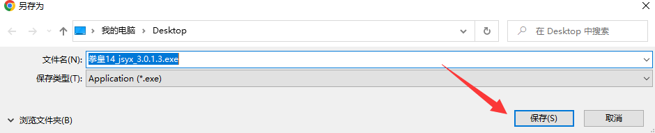
5.
点击保存即可
- 上一篇:魔兽争霸3下载官方(魔兽争霸3下载官方网站)
- 下一篇:使命召唤16单机版中文破解版
相关推荐
- 晚清特种狙击手(清朝狙击枪)
-
清朝万大军奔赴前线,到了战场发现对手不是人,最终一败涂地转眼到了一百多年后的弘历当政时期,大内深处传出一阵掀翻屋顶的咆哮声。乾隆指着那帮灰头土脸回京的将领,唾沫星子乱飞,直骂他们活得还没牲口明白。这位...
- 全娱乐圈颤抖(全娱乐圈颤抖by林知落)
-
唐国强一语成谶!演艺圈迎来至暗时刻,AI抢饭碗,谁在瑟瑟发抖?谁曾想,去年唐国强在节目里那句被当成笑话的“AI会取代人类演员”,如今竟一语成谶,成了悬在无数演艺人员头顶的达摩克利斯之剑。年两会刚落幕一...
- 龙腾宇内全文阅读(龙腾宇内小说免费下载)
-
十大种马后宫文小说〖引言〗龙马:古代传说中形态像龙的骏马。语出唐o李郢《上裴晋公》诗:“四朝忧国鬓如丝,龙马精神海鸥姿。”龙马精神指像龙马那样精神焕发,形容人的精神健旺充沛、斗志昂扬,多用来称赞人饱满...
- 经年后钟情如初(经年后钟情如初简安安)
-
认定了你,钟情你,偏爱你,就是一辈子!作者:赴梦青孤光阴的故事里,总有一阵风,吹老了芳华,却为人生增加一抹馨香,那是人世间的别样风情,是定格在心中的情感。置身于幽深的红尘里,有一种遇见,一旦开始,就...
- 江瑟瑟靳封臣全文免费阅读(江瑟瑟靳封臣列表免费阅读)
-
书单高评分高质量本霸道总裁小说合集靳封臣愣了愣,看了她一眼,似有些犹豫,不过很快便点了头。江瑟瑟上前两步,敲了敲门,对屋内的小家伙道:“宝贝儿,菜饭都做好了,再不吃就要凉了,你出来好不好?”屋内传来...
- 重生80从民办教师做起(重生80从民办教师做起 第137章)
-
五部讲台上的爽文制造机:支教、实习、班主任、民办、代课全覆盖人民城市的“双率先”密码——上海持续推进基础教育优质均衡普惠观察在超大城市治理的复杂棋局中,基础教育优质均衡普惠,何以成为人民城市的鲜明底...
- 洪荒之亘古(洪荒之亘古txt全集)
-
山河赋.十五首庐山,就在不远的前方我看见了,彩虹另一端的指向,山的那一边。我看见了原野的辽远,唯有“高处不胜寒”栅栏的终结。凭高俯览,群峰耸立,岩壁峭拔,千峰拥翠;淡淡晨雾,悬在峰峦之巅。动中...
- 明末之领主天下(明末之领主天下百度百科)
-
《天启异闻录》:西方的怪兽,无法讲好中国的故事撰文丨波音摘编丨何安安大一统的中国是怎么来的?后金–清的勃兴是怎样发生的?它的出现对于中华文明的融合进程又产生了怎样的影响?以草原文明的视角来看待中华民族...
- 重生之矿业巨头(重生之矿业巨头TXT下载)
-
北京程序员投万紫金矿业,年赚万,见证矿业巨头崛起!有人盯着一家公司的一串数字看了很久,最先注意到的不是营收,也不是市值,而是现金流,能把钱稳稳收回来的企业,往往更能扛住风浪另一个人只看产量,他说矿业不...
- 华娱大时代(华娱大时代唐安)
-
三本高质量的文娱后宫文,车速够快,喜欢多女主的书友别错过大家好,我是小胖。今天小胖给大家推荐几本高质量的都市类娱乐后宫文,多女主,车速够快,喜欢这类题材的小伙伴不要错过。《火爆天王》作者:柳下惠类型:...
- 灵师 暗夜萧然(灵师暗夜萧然百度百科)
-
《穿越兽世之夫君恋爱脑控制一下》元珈罗阿瓦达完结版阅读在信息过载、焦虑蔓延的当下,人总在寻找各种“心灵解药”。最近,笔者意外地发现晚间观看历史人文传记类纪录片,竟有助安神。从《李白》《苏东坡》,到《人...
- 重生空间之军宠闲妻(重生空间之军婚盛宠)
-
本陈三爷同款男主,权倾朝野+禁欲腹黑+深情偏执+宠妻无度《盛世嫡妃》聪明伶俐重生女&冷酷腹黑深情王爷“本王不信鬼神,不求苍天。她若殒命,本王便将这天下化为炼狱,让这山河为她作祭!”男强女强,但...
- 亵渎txt下载全文下载(亵渎之鳞txt)
-
微言|一年本?“伪读书”闹剧该收场了■刘云生年5月,江苏沭阳两位老人在儿子提供的居住屋内支了灶台做饭。儿子和儿媳认为主屋内支灶台不仅有碍观瞻,还有安全隐患,要求父母拆除,被拒绝后小两口直接将灶台...
- 医仙门(医仙门诊)
-
小说:医仙门少主成废物赘婿,病人病危,他一招搞定,众人傻眼一只蝴蝶[宇宙一片白茫茫的,真干净…… 蝉噪风秋,山月勾悬。 月光泻如银河水,将整个湖面照亮。 这死水一片,远眺高低错落无数玉枝,近...
- 总裁的天价小妻子 韩降雪 小说
-
美国得克萨斯州电价疯涨,一女子收到7万多元“天价”电费单来源:环球网【环球网报道记者侯佳欣】罕见的冬季风暴日前造成美国南部得克萨斯州多处停电、停水。此外,部分生活必需品和电价也出现暴涨。据“今日俄...
- 一周热门


- 最近发表
- 标签列表
-